Processing and Epoching Pupil Size Data#

When working with event-based recordings, it’s often useful to extract and analyze data segments surrounding those events, rather than processing the entire recording. In mobile eye-tracking, such events could include stimulus presentations or the participant entering a specific area. In this tutorial, we’ll demonstrate how to epoch data around these events using the pyneon.Epochs class, with the sample recording PLR.

[1]:

from pyneon import Dataset, get_sample_data

# Create a Recording object
dataset_dir = get_sample_data("PLR", format="native")
dataset = Dataset(dataset_dir)
rec = dataset.recordings[0]
scene_video = rec.scene_video
blinks = rec.blinks
events = rec.events
eye_states = rec.eye_states

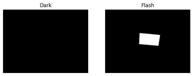
This recording features a participant observing a screen that flashes from black to white (flash duration = 0.75 s), with a 3-second interval between flashes. We expect the pupil to constrict in response to each flash, making this dataset ideal for demonstrating epoching. Here is how the flash appears to the participant:

[2]:

import matplotlib.pyplot as plt

# Create a figure
fig, axs = plt.subplots(1, 2, figsize=(8, 3))

# Visualize two frames from the video that correspond to the dark and flash periods
scene_video.plot_frame(150, ax=axs[0], show=False)
scene_video.plot_frame(200, ax=axs[1], show=False)
axs[0].set_title("Dark")
axs[1].set_title("Flash")
plt.show()

../_images/tutorials_pupil_size_and_epoching_3_0.png

[3]:

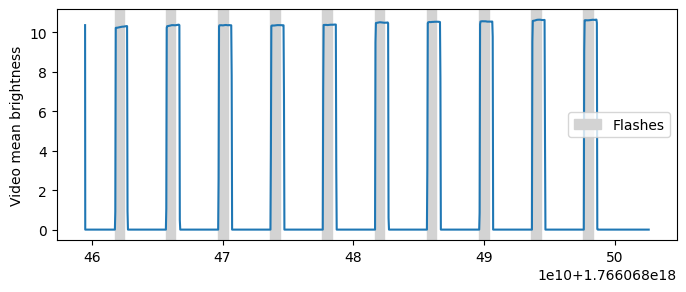
# Filter events to get flash onsets
flashes = events.filter_by_name("flash onset")
print(flashes.data)

# # Compute video frame intensities
intensities = scene_video.compute_frame_brightness()
plt.figure(figsize=(8, 3))
plt.plot(intensities["brightness"])
for onset in flashes.start_ts:
    dur = plt.axvspan(
        onset, onset + 0.75 * 1e9, color="lightgray", label="Flashes"
    )  # Each flash lasts 2 seconds
plt.ylabel("Video mean brightness")
plt.legend(handles=[dur])
plt.show()

               timestamp [ns]         name       type
event id
1         1766068461745390000  flash onset  recording
2         1766068465647497000  flash onset  recording
3         1766068469642822000  flash onset  recording
4         1766068473635128000  flash onset  recording
5         1766068477629326000  flash onset  recording
6         1766068481628174000  flash onset  recording
7         1766068485617192000  flash onset  recording
8         1766068489611285000  flash onset  recording
9         1766068493606366000  flash onset  recording
10        1766068497595856000  flash onset  recording

Computing frame brightness: 100%|██████████| 1295/1295 [00:10<00:00, 124.41it/s]

../_images/tutorials_pupil_size_and_epoching_4_2.png

Visualizing raw pupil size data and repairing blink artifacts#

Let’s inspect the raw pupil size data along with blink events. The shaded region shows when the screen is bright; dashed lines indicate the onset of blinks.

[4]:

plt.figure(figsize=(8, 3))

# Visualize the flashes
for flash_start in flashes.start_ts:
    dur = plt.axvspan(
        flash_start, flash_start + 0.75 * 1e9, color="lightgray", label="Flashes"
    )  # Each flash lasts 2 seconds

# Visualize the blinks
for blink_start in blinks.start_ts:
    line = plt.axvline(blink_start, color="k", linestyle="--", lw=1, label="Blinks")

# Plot the pupil data
(pupil_l,) = plt.plot(eye_states["pupil diameter right [mm]"])

plt.xlabel("Timestamp [ns]")
plt.ylabel("Left pupil diameter [mm]")
plt.legend(handles=[dur, line])
plt.show()

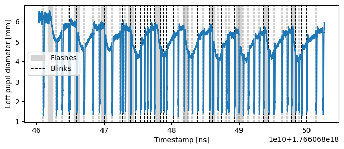
../_images/tutorials_pupil_size_and_epoching_6_0.png

From the plot we can note:

Pupil size decreases promptly after each change in screen brightness.
The participant frequently blinks in response to flashes, and blinks introduce distinct transient artifacts in the pupil size measurement.

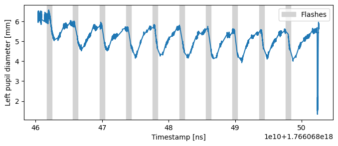
First, we’ll address blink artifacts using the interpolate_events() method of the Stream class. This method masks the data during events (in this case, blinks) and interpolates values around them, effectively removing the transient artifacts.

[5]:

eye_states.interpolate_events(blinks, inplace=True)

plt.figure(figsize=(8, 3))

# Visualize the flashes
for flash_start in flashes.start_ts:
    dur = plt.axvspan(
        flash_start, flash_start + 7.5 * 1e8, color="lightgray", label="Flashes"
    )  # Each flash lasts 2 seconds

# Plot the pupil data
(pupil_l,) = plt.plot(eye_states["pupil diameter right [mm]"])

plt.xlabel("Timestamp [ns]")
plt.ylabel("Left pupil diameter [mm]")
plt.legend(handles=[dur])
plt.show()

../_images/tutorials_pupil_size_and_epoching_8_0.png

Defining Epochs: Creating the `epochs_info` DataFrame#

In order to perform epoching, we require information about the timing and length of epochs. Explicitly, every epoch requires:

A reference time t_ref
A time window defined by t_before and t_after to extract the data from
An event description to annotate the epoch.

PyNeon’s Epochs implementation allows epochs of variable lengths, where t_before and t_after may differ for each event. As a result, defining all epochs requires a DataFrame (epochs_info) with columns: t_ref, t_before, t_after, and description.

While constructing such a DataFrame by hand is possible, it’s easier to generate one using event information from PyNeon Events objects. The events_to_epochs_info function streamlines this process by using the onsets of events and user-defined t_before/t_after values.

In this example, we’ll use "flash onset" events, extracting 0.5 seconds before to 3 seconds after each event; the description is set to the event name automatically.

[6]:

from pyneon import Epochs, events_to_epochs_info

# For complex events, such as those from `events.csv`, we need to specify the event name
flash_epochs_info = events_to_epochs_info(
    events, t_before=0.5, t_after=3, t_unit="s", event_name="flash onset"
)

# Print the epoching-ready epochs_info
print("\nFlash times DataFrame:")
print(flash_epochs_info.head())


Flash times DataFrame:
                 t_ref   t_before     t_after  description
0  1766068461745390000  500000000  3000000000  flash onset
1  1766068465647497000  500000000  3000000000  flash onset
2  1766068469642822000  500000000  3000000000  flash onset
3  1766068473635128000  500000000  3000000000  flash onset
4  1766068477629326000  500000000  3000000000  flash onset

Creating `Epochs` objects#

With the epochs_info DataFrame, we can create epochs by passing it along with the relevant Stream or Events data to the Epochs class.

In this example, we create two types of epochs to test two hypotheses:

eye_ep: epochs from eye_states (a Stream object), containing pupil size. We hypothesize pupil size will decrease after each flash.
blink_ep: epochs from blinks (an Events object), letting us check if blinks cluster after each flash.

[7]:

eye_ep = Epochs(eye_states, flash_epochs_info)
blink_ep = Epochs(blinks, flash_epochs_info)
imu_ep = Epochs(rec.imu, flash_epochs_info)
print(f"{len(eye_ep)} epochs created from {len(flash_epochs_info)} events")

10 epochs created from 10 events

Given that we have very sparse blink events, it is not surprising that PyNeon emits a warning when creating the blink_ep epochs.

The Epochs class provides two key attributes (for details, see the API reference):

epochs_dict: a dictionary keyed by epoch index; each value is a Stream or Events instance (or None if empty), with an added epoch time [ns] column.
epochs_info: the DataFrame describing t_ref, t_before, t_after, and description, plus derived t_start and t_end.

For quick inspection, Epochs.data returns the first non-empty epoch’s DataFrame, but analysis should use epochs_dict and epochs_info.

[8]:

epochs = eye_ep.epochs_dict
print(f"epochs is a {type(epochs)} with {len(epochs)} items.")
first_epoch = epochs[0]
print(f"Dict values are {type(first_epoch)} with shape {first_epoch.data.shape}.")

epochs_info = eye_ep.epochs_info
print(epochs_info.index)

epochs is a <class 'dict'> with 10 items.
Dict values are <class 'pyneon.stream.Stream'> with shape (699, 21).
RangeIndex(start=0, stop=10, step=1, name='epoch index')

Visualizing epoch data#

The plot() method provides a convenient way to visualize data across epochs.

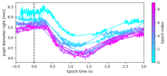
For Epochs created from a Stream (like eye states), specify the desired column to plot the same variable across epochs in a single figure, colored by epoch index. We can observe from the following plot that pupil constriction occurs after each flash consistently, except for the first flash, likely due to a different baseline pupil size.

[9]:

fig, ax = plt.subplots(figsize=(8, 3))
fig, ax = eye_ep.plot("pupil diameter right [mm]", ax=ax)

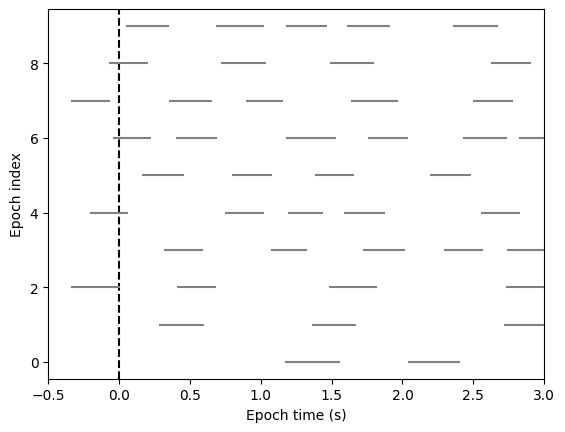
../_images/tutorials_pupil_size_and_epoching_16_0.png

For Events-based Epochs (like blinks), simply call plot() with no arguments. Here, each event is displayed as a horizontal line spanning its duration, vertically sorted by epoch. We can see that blinks (N=4 in this example) tend to happen 1 to 1.5 seconds after each flash.

[10]:

fig, ax = blink_ep.plot()

../_images/tutorials_pupil_size_and_epoching_18_0.png

Converting `Stream`-based `Epochs` to a Numpy array#

Rather than viewing epochs as nested DataFrames, under the right conditions, you can convert an Epochs object to a 3D NumPy array useful for time-series analyses (like with MNE-Python).

For this:

The source must be a uniformly sampled Stream (constant intervals between samples).
All epochs must have the same durations (t_before and t_after equal).

If these are not met, PyNeon will raise a ValueError when to_numpy() is called.

To ensure compatibility, interpolate the Stream data prior to epoching, and maintain constant window sizes across epochs. The resulting array will be shaped (n_epochs, n_channels, n_times).

[11]:

# Create an epoch with the interpolated data
epochs_np, info = eye_ep.to_numpy()

print(f"(n_epochs, n_channels, n_times) = {epochs_np.shape}")
print(info)

(n_epochs, n_channels, n_times) = (10, 20, 700)
{'epoch_times': array([-500000000, -495000000, -490000000, -485000000, -480000000,
       -475000000, -470000000, -465000000, -460000000, -455000000,
       -450000000, -445000000, -440000000, -435000000, -430000000,
       -425000000, -420000000, -415000000, -410000000, -405000000,
       -400000000, -395000000, -390000000, -385000000, -380000000,
       -375000000, -370000000, -365000000, -360000000, -355000000,
       -350000000, -345000000, -340000000, -335000000, -330000000,
       -325000000, -320000000, -315000000, -310000000, -305000000,
       -300000000, -295000000, -290000000, -285000000, -280000000,
       -275000000, -270000000, -265000000, -260000000, -255000000,
       -250000000, -245000000, -240000000, -235000000, -230000000,
       -225000000, -220000000, -215000000, -210000000, -205000000,
       -200000000, -195000000, -190000000, -185000000, -180000000,
       -175000000, -170000000, -165000000, -160000000, -155000000,
       -150000000, -145000000, -140000000, -135000000, -130000000,
       -125000000, -120000000, -115000000, -110000000, -105000000,
       -100000000,  -95000000,  -90000000,  -85000000,  -80000000,
        -75000000,  -70000000,  -65000000,  -60000000,  -55000000,
        -50000000,  -45000000,  -40000000,  -35000000,  -30000000,
        -25000000,  -20000000,  -15000000,  -10000000,   -5000000,
                0,    5000000,   10000000,   15000000,   20000000,
         25000000,   30000000,   35000000,   40000000,   45000000,
         50000000,   55000000,   60000000,   65000000,   70000000,
         75000000,   80000000,   85000000,   90000000,   95000000,
        100000000,  105000000,  110000000,  115000000,  120000000,
        125000000,  130000000,  135000000,  140000000,  145000000,
        150000000,  155000000,  160000000,  165000000,  170000000,
        175000000,  180000000,  185000000,  190000000,  195000000,
        200000000,  205000000,  210000000,  215000000,  220000000,
        225000000,  230000000,  235000000,  240000000,  245000000,
        250000000,  255000000,  260000000,  265000000,  270000000,
        275000000,  280000000,  285000000,  290000000,  295000000,
        300000000,  305000000,  310000000,  315000000,  320000000,
        325000000,  330000000,  335000000,  340000000,  345000000,
        350000000,  355000000,  360000000,  365000000,  370000000,
        375000000,  380000000,  385000000,  390000000,  395000000,
        400000000,  405000000,  410000000,  415000000,  420000000,
        425000000,  430000000,  435000000,  440000000,  445000000,
        450000000,  455000000,  460000000,  465000000,  470000000,
        475000000,  480000000,  485000000,  490000000,  495000000,
        500000000,  505000000,  510000000,  515000000,  520000000,
        525000000,  530000000,  535000000,  540000000,  545000000,
        550000000,  555000000,  560000000,  565000000,  570000000,
        575000000,  580000000,  585000000,  590000000,  595000000,
        600000000,  605000000,  610000000,  615000000,  620000000,
        625000000,  630000000,  635000000,  640000000,  645000000,
        650000000,  655000000,  660000000,  665000000,  670000000,
        675000000,  680000000,  685000000,  690000000,  695000000,
        700000000,  705000000,  710000000,  715000000,  720000000,
        725000000,  730000000,  735000000,  740000000,  745000000,
        750000000,  755000000,  760000000,  765000000,  770000000,
        775000000,  780000000,  785000000,  790000000,  795000000,
        800000000,  805000000,  810000000,  815000000,  820000000,
        825000000,  830000000,  835000000,  840000000,  845000000,
        850000000,  855000000,  860000000,  865000000,  870000000,
        875000000,  880000000,  885000000,  890000000,  895000000,
        900000000,  905000000,  910000000,  915000000,  920000000,
        925000000,  930000000,  935000000,  940000000,  945000000,
        950000000,  955000000,  960000000,  965000000,  970000000,
        975000000,  980000000,  985000000,  990000000,  995000000,
       1000000000, 1005000000, 1010000000, 1015000000, 1020000000,
       1025000000, 1030000000, 1035000000, 1040000000, 1045000000,
       1050000000, 1055000000, 1060000000, 1065000000, 1070000000,
       1075000000, 1080000000, 1085000000, 1090000000, 1095000000,
       1100000000, 1105000000, 1110000000, 1115000000, 1120000000,
       1125000000, 1130000000, 1135000000, 1140000000, 1145000000,
       1150000000, 1155000000, 1160000000, 1165000000, 1170000000,
       1175000000, 1180000000, 1185000000, 1190000000, 1195000000,
       1200000000, 1205000000, 1210000000, 1215000000, 1220000000,
       1225000000, 1230000000, 1235000000, 1240000000, 1245000000,
       1250000000, 1255000000, 1260000000, 1265000000, 1270000000,
       1275000000, 1280000000, 1285000000, 1290000000, 1295000000,
       1300000000, 1305000000, 1310000000, 1315000000, 1320000000,
       1325000000, 1330000000, 1335000000, 1340000000, 1345000000,
       1350000000, 1355000000, 1360000000, 1365000000, 1370000000,
       1375000000, 1380000000, 1385000000, 1390000000, 1395000000,
       1400000000, 1405000000, 1410000000, 1415000000, 1420000000,
       1425000000, 1430000000, 1435000000, 1440000000, 1445000000,
       1450000000, 1455000000, 1460000000, 1465000000, 1470000000,
       1475000000, 1480000000, 1485000000, 1490000000, 1495000000,
       1500000000, 1505000000, 1510000000, 1515000000, 1520000000,
       1525000000, 1530000000, 1535000000, 1540000000, 1545000000,
       1550000000, 1555000000, 1560000000, 1565000000, 1570000000,
       1575000000, 1580000000, 1585000000, 1590000000, 1595000000,
       1600000000, 1605000000, 1610000000, 1615000000, 1620000000,
       1625000000, 1630000000, 1635000000, 1640000000, 1645000000,
       1650000000, 1655000000, 1660000000, 1665000000, 1670000000,
       1675000000, 1680000000, 1685000000, 1690000000, 1695000000,
       1700000000, 1705000000, 1710000000, 1715000000, 1720000000,
       1725000000, 1730000000, 1735000000, 1740000000, 1745000000,
       1750000000, 1755000000, 1760000000, 1765000000, 1770000000,
       1775000000, 1780000000, 1785000000, 1790000000, 1795000000,
       1800000000, 1805000000, 1810000000, 1815000000, 1820000000,
       1825000000, 1830000000, 1835000000, 1840000000, 1845000000,
       1850000000, 1855000000, 1860000000, 1865000000, 1870000000,
       1875000000, 1880000000, 1885000000, 1890000000, 1895000000,
       1900000000, 1905000000, 1910000000, 1915000000, 1920000000,
       1925000000, 1930000000, 1935000000, 1940000000, 1945000000,
       1950000000, 1955000000, 1960000000, 1965000000, 1970000000,
       1975000000, 1980000000, 1985000000, 1990000000, 1995000000,
       2000000000, 2005000000, 2010000000, 2015000000, 2020000000,
       2025000000, 2030000000, 2035000000, 2040000000, 2045000000,
       2050000000, 2055000000, 2060000000, 2065000000, 2070000000,
       2075000000, 2080000000, 2085000000, 2090000000, 2095000000,
       2100000000, 2105000000, 2110000000, 2115000000, 2120000000,
       2125000000, 2130000000, 2135000000, 2140000000, 2145000000,
       2150000000, 2155000000, 2160000000, 2165000000, 2170000000,
       2175000000, 2180000000, 2185000000, 2190000000, 2195000000,
       2200000000, 2205000000, 2210000000, 2215000000, 2220000000,
       2225000000, 2230000000, 2235000000, 2240000000, 2245000000,
       2250000000, 2255000000, 2260000000, 2265000000, 2270000000,
       2275000000, 2280000000, 2285000000, 2290000000, 2295000000,
       2300000000, 2305000000, 2310000000, 2315000000, 2320000000,
       2325000000, 2330000000, 2335000000, 2340000000, 2345000000,
       2350000000, 2355000000, 2360000000, 2365000000, 2370000000,
       2375000000, 2380000000, 2385000000, 2390000000, 2395000000,
       2400000000, 2405000000, 2410000000, 2415000000, 2420000000,
       2425000000, 2430000000, 2435000000, 2440000000, 2445000000,
       2450000000, 2455000000, 2460000000, 2465000000, 2470000000,
       2475000000, 2480000000, 2485000000, 2490000000, 2495000000,
       2500000000, 2505000000, 2510000000, 2515000000, 2520000000,
       2525000000, 2530000000, 2535000000, 2540000000, 2545000000,
       2550000000, 2555000000, 2560000000, 2565000000, 2570000000,
       2575000000, 2580000000, 2585000000, 2590000000, 2595000000,
       2600000000, 2605000000, 2610000000, 2615000000, 2620000000,
       2625000000, 2630000000, 2635000000, 2640000000, 2645000000,
       2650000000, 2655000000, 2660000000, 2665000000, 2670000000,
       2675000000, 2680000000, 2685000000, 2690000000, 2695000000,
       2700000000, 2705000000, 2710000000, 2715000000, 2720000000,
       2725000000, 2730000000, 2735000000, 2740000000, 2745000000,
       2750000000, 2755000000, 2760000000, 2765000000, 2770000000,
       2775000000, 2780000000, 2785000000, 2790000000, 2795000000,
       2800000000, 2805000000, 2810000000, 2815000000, 2820000000,
       2825000000, 2830000000, 2835000000, 2840000000, 2845000000,
       2850000000, 2855000000, 2860000000, 2865000000, 2870000000,
       2875000000, 2880000000, 2885000000, 2890000000, 2895000000,
       2900000000, 2905000000, 2910000000, 2915000000, 2920000000,
       2925000000, 2930000000, 2935000000, 2940000000, 2945000000,
       2950000000, 2955000000, 2960000000, 2965000000, 2970000000,
       2975000000, 2980000000, 2985000000, 2990000000, 2995000000]), 'column_names': ['pupil diameter left [mm]', 'eyeball center left x [mm]', 'eyeball center left y [mm]', 'eyeball center left z [mm]', 'optical axis left x', 'optical axis left y', 'optical axis left z', 'pupil diameter right [mm]', 'eyeball center right x [mm]', 'eyeball center right y [mm]', 'eyeball center right z [mm]', 'optical axis right x', 'optical axis right y', 'optical axis right z', 'eyelid angle top left [rad]', 'eyelid angle bottom left [rad]', 'eyelid aperture left [mm]', 'eyelid angle top right [rad]', 'eyelid angle bottom right [rad]', 'eyelid aperture right [mm]'], 'nan_flag': np.False_}

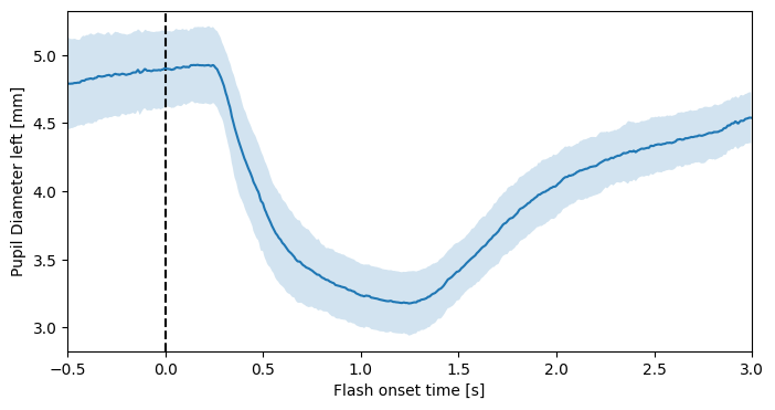
In this case, we have 10 epochs, 20 data channels, and 699 time steps—consistent with the 200 Hz sampling rate and the 3.5-second epoch window. The info object contains lists of column IDs and epoch times. Now, the grand average is easily computed:

[12]:

# Average the first channel (pupil diameter right [mm]) across all epochs
epoch_times = info["epoch_times"] / 1e9
pupil_mean = epochs_np[:, 0, :].mean(axis=0)
pupil_std = epochs_np[:, 0, :].std(axis=0)

plt.figure(figsize=(8, 4))

# Show a vertical line at 0
plt.axvline(x=0, color="k", linestyle="--")
# Plot the mean pupil diameter and standard deviation
plt.plot(epoch_times, pupil_mean)
plt.fill_between(epoch_times, pupil_mean - pupil_std, pupil_mean + pupil_std, alpha=0.2)
plt.xlim(-0.5, 3)
plt.xlabel("flash onset time [s]")
plt.ylabel("pupil diameter right [mm]")
plt.show()

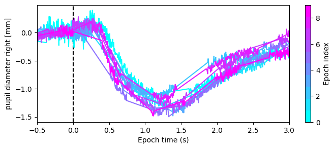
../_images/tutorials_pupil_size_and_epoching_23_0.png

Baseline correction#

Optionally, apply apply_baseline() to reduce global fluctuations in the data. The default method="mean" subtracts the mean of a pre-event baseline window. If there is a linear trend in the baseline, method="regression" fits and removes it across the epoch.

Here, we apply apply_baseline() with method="mean" to compare pupil size relative to a 500 ms pre-flash baseline, centering pre-flash values around zero and reducing variance.

[13]:

eye_ep.apply_baseline(
    baseline=(-0.5, 0),
    method="mean",
)
fig, ax = plt.subplots(figsize=(8, 3))
eye_ep.plot("pupil diameter right [mm]", ax=ax)

../_images/tutorials_pupil_size_and_epoching_25_0.png

[13]:

(<Figure size 800x300 with 2 Axes>,
 <Axes: xlabel='Epoch time (s)', ylabel='pupil diameter right [mm]'>)

Processing and Epoching Pupil Size Data#

Visualizing raw pupil size data and repairing blink artifacts#

Defining Epochs: Creating the epochs_info DataFrame#

Creating Epochs objects#

Visualizing epoch data#

Converting Stream-based Epochs to a Numpy array#

Baseline correction#

This Page

Defining Epochs: Creating the `epochs_info` DataFrame#

Creating `Epochs` objects#

Converting `Stream`-based `Epochs` to a Numpy array#