Reading a Neon dataset/recording#
In this tutorial, we will show how to load a single Neon recording downloaded from Pupil Cloud and give an overview of the data structure.
Reading sample data#
We will use a sample recording produced by the NCC Lab, called boardView. This project (collection of recordings on Pupil Cloud) contains two recordings downloaded with the Timeseries Data + Scene Video option and a marker mapper enrichment. It can be downloaded with the get_sample_data() function. The function returns a Pathlib.Path (reference) instance pointing to the downloaded and unzipped directory. PyNeon
accepts both Path and string objects but internally always uses Path.
[1]:
from pyneon import get_sample_data, Dataset, Recording

# Download sample data (if not existing) and return the path
sample_dir = get_sample_data("boardView")
print(sample_dir)
C:\Users\qian.chu\Documents\GitHub\PyNeon\data\boardView
The OfficeWalk data has the following structure:
boardView
├── Timeseries Data + Scene Video
│   ├── boardview1-d4fd9a27
│   │   ├── info.json
│   │   ├── gaze.csv
│   │   └── ....
│   ├── boardview2-713532d5
│   │   ├── info.json
│   │   ├── gaze.csv
│   │   └── ....
|   ├── enrichment_info.txt
|   └── sections.csv
└── boardView_MARKER-MAPPER_boardMapping_csv
The Timeseries Data + Scene Video folder contains what PyNeon refers to as a Dataset. It consists of two recordings, each with its own info.json file and data files. These recordings can be loaded either individually as a Recording, or as a collective Dataset.
To load a Dataset, specify the path to the Timeseries Data + Scene Video folder:
[2]:
dataset_dir = sample_dir / "Timeseries Data + Scene Video"
dataset = Dataset(dataset_dir)
print(dataset)
Dataset | 2 recordings
Dataset provides an index-based access to its recordings. The recordings are stored in the recordings attribute, which contains a list of Recording instances. You can access individual recordings by index:
[3]:
rec = dataset[0]  # Internally accesses the recordings attribute
print(type(rec))
print(rec.recording_dir)
<class 'pyneon.recording.Recording'>
C:\Users\qian.chu\Documents\GitHub\PyNeon\data\boardView\Timeseries Data + Scene Video\boardview2-713532d5
Alternatively, you can directly load a single Recording by specifying the recording’s folder path:
[4]:
recording_dir = dataset_dir / "boardview1-d4fd9a27"
rec = Recording(recording_dir)
print(type(rec))
print(rec.recording_dir)
<class 'pyneon.recording.Recording'>
C:\Users\qian.chu\Documents\GitHub\PyNeon\data\boardView\Timeseries Data + Scene Video\boardview1-d4fd9a27
Data and metadata of a Recording#
You can quickly get an overview of the metadata and contents of a Recording by printing the instance. The basic metadata (e.g., recording and wearer ID, recording start time and duration) and the path to available data will be displayed. At this point, the data is simply located from the recording’s folder path, but it is not yet loaded into memory.
[5]:
print(rec)
Recording ID: d4fd9a27-3e28-45bf-937f-b9c14c3c1c5e
Wearer ID: af6cd360-443a-4d3d-adda-7dc8510473c2
Wearer name: Qian
Recording start time: 2024-11-26 12:44:48.937000
Recording duration: 32.046s
                 exist                 filename                                                                                                                                path
3d_eye_states     True        3d_eye_states.csv        C:\Users\qian.chu\Documents\GitHub\PyNeon\data\boardView\Timeseries Data + Scene Video\boardview1-d4fd9a27\3d_eye_states.csv
blinks            True               blinks.csv               C:\Users\qian.chu\Documents\GitHub\PyNeon\data\boardView\Timeseries Data + Scene Video\boardview1-d4fd9a27\blinks.csv
events            True               events.csv               C:\Users\qian.chu\Documents\GitHub\PyNeon\data\boardView\Timeseries Data + Scene Video\boardview1-d4fd9a27\events.csv
fixations         True            fixations.csv            C:\Users\qian.chu\Documents\GitHub\PyNeon\data\boardView\Timeseries Data + Scene Video\boardview1-d4fd9a27\fixations.csv
gaze              True                 gaze.csv                 C:\Users\qian.chu\Documents\GitHub\PyNeon\data\boardView\Timeseries Data + Scene Video\boardview1-d4fd9a27\gaze.csv
imu               True                  imu.csv                  C:\Users\qian.chu\Documents\GitHub\PyNeon\data\boardView\Timeseries Data + Scene Video\boardview1-d4fd9a27\imu.csv
labels            True               labels.csv               C:\Users\qian.chu\Documents\GitHub\PyNeon\data\boardView\Timeseries Data + Scene Video\boardview1-d4fd9a27\labels.csv
saccades          True             saccades.csv             C:\Users\qian.chu\Documents\GitHub\PyNeon\data\boardView\Timeseries Data + Scene Video\boardview1-d4fd9a27\saccades.csv
world_timestamps  True     world_timestamps.csv     C:\Users\qian.chu\Documents\GitHub\PyNeon\data\boardView\Timeseries Data + Scene Video\boardview1-d4fd9a27\world_timestamps.csv
scene_video_info  True        scene_camera.json        C:\Users\qian.chu\Documents\GitHub\PyNeon\data\boardView\Timeseries Data + Scene Video\boardview1-d4fd9a27\scene_camera.json
scene_video       True  182240fd_0.0-32.046.mp4  C:\Users\qian.chu\Documents\GitHub\PyNeon\data\boardView\Timeseries Data + Scene Video\boardview1-d4fd9a27\182240fd_0.0-32.046.mp4
As seen in the output, this recording includes all data files. This tutorial will focus on non-video data. For processing video, refer to the Neon video tutorial.
Individual data streams can be accessed as properties of the Recording instance. For example, the gaze data can be accessed as recording.gaze, and upon accessing, the tabular data is loaded into memory. On the other hand, if you try to access unavailable data, PyNeon will return None and a warning message.
[6]:
# Gaze and fixation data are available
gaze = rec.gaze
print(f"recording.gaze is {gaze}")

saccades = rec.saccades
print(f"recording.saccades is {saccades}")

video = rec.video
print(f"recording.video is {video}")
recording.gaze is <pyneon.stream.Stream object at 0x000002A59ECFC980>
recording.saccades is <pyneon.events.Events object at 0x000002A59ECFC590>
recording.video is < cv2.VideoCapture 000002A5C052BA10>
PyNeon reads tabular CSV file into specialized classes (e.g., gaze.csv to NeonGaze) which all have a data attribute that holds the tabular data as a pandas.DataFrame (reference). Depending on the nature of the data, such classes could be of Stream or Events super classes. Stream contains (semi)-continuous data streams, while Events (dubbed so to avoid confusion with the
Eventsent subclass that holds data from events.csv) contains sparse event data.
The class inheritance relationship is as follows:
NeonTabular
├── Stream
│   ├── NeonGaze
│   ├── NeonEyeStates
│   └── NeonIMU
└── Events
    ├── NeonBlinks
    ├── NeonSaccades
    ├── NeonFixations
    └── Eventsents
Data as DataFrames#
The essence of NeonTabular is the data attribute—a pandas.DataFrame. This is a common data structure in Python for handling tabular data. For example, you can print the first 5 rows of the gaze data by calling gaze.data.head(), and inspect the data type of each column by calling gaze.data.dtypes.
Theoretically, you could re-assign gaze.data to gaze_df, however the conversion scripts written in the next section only work at the class level and not on the dataframe level.
[7]:
print(gaze.data.head())
print(gaze.data.dtypes)
                     gaze x [px]  gaze y [px]  worn  fixation id  blink id  \
timestamp [ns]
1732621490425631343      697.829      554.242     1            1      <NA>
1732621490430625343      698.096      556.335     1            1      <NA>
1732621490435625343      697.810      556.360     1            1      <NA>
1732621490440625343      695.752      557.903     1            1      <NA>
1732621490445625343      696.108      558.438     1            1      <NA>

                     azimuth [deg]  elevation [deg]
timestamp [ns]
1732621490425631343      -7.581023         3.519804
1732621490430625343      -7.563214         3.385485
1732621490435625343      -7.581576         3.383787
1732621490440625343      -7.713686         3.284294
1732621490445625343      -7.690596         3.250055
gaze x [px]        float64
gaze y [px]        float64
worn                 Int32
fixation id          Int32
blink id             Int32
azimuth [deg]      float64
elevation [deg]    float64
dtype: object
[8]:
print(saccades.data.head())
print(saccades.data.dtypes)
                      saccade id   end timestamp [ns]  duration [ms]  \
start timestamp [ns]
1732621490876132343            1  1732621490891115343             15
1732621491241357343            2  1732621491291481343             50
1732621491441602343            3  1732621491516601343             75
1732621491626723343            4  1732621491696847343             70
1732621491917092343            5  1732621491977090343             60

                      amplitude [px]  amplitude [deg]  mean velocity [px/s]  \
start timestamp [ns]
1732621490876132343        14.938179         0.962102           1025.709879
1732621491241357343       130.743352         8.378644           2700.713283
1732621491441602343       241.003342        15.391730           3615.380044
1732621491626723343       212.619205        13.608618           3757.394092
1732621491917092343       220.842812        13.914266           4220.180601

                      peak velocity [px/s]
start timestamp [ns]
1732621490876132343            1191.520740
1732621491241357343            3687.314947
1732621491441602343            5337.244676
1732621491626723343            6164.040944
1732621491917092343            6369.217052
saccade id                Int32
end timestamp [ns]        Int64
duration [ms]             Int64
amplitude [px]          float64
amplitude [deg]         float64
mean velocity [px/s]    float64
peak velocity [px/s]    float64
dtype: object
PyNeon performs the following preprocessing when reading the CSV files:
Removes the redundant
section idandrecording idcolumns that are present in the raw CSVs.Sets the
timestamp [ns](orstart timestamp [ns]for most event files) column as the DataFrame index.Automatically assigns appropriate data types to columns. For instance,
Int64type is assigned to timestamps,Int32to event IDs (blink/fixation/saccade ID), andfloat64to float data (e.g. gaze location, pupil size).
Just like any other pandas.DataFrame, you can access individual rows, columns, or subsets of the data using the standard indexing and slicing methods. For example, gaze.data.iloc[0] returns the first row of the gaze data, and gaze.data['gaze x [px]'] (or gaze['gaze x [px]']) returns the gaze x-coordinate column.
[9]:
print(f"First row of gaze data:\n{gaze.data.iloc[0]}\n")
print(f"All gaze x values:\n{gaze['gaze x [px]']}")
First row of gaze data:
gaze x [px]         697.829
gaze y [px]         554.242
worn                    1.0
fixation id             1.0
blink id               <NA>
azimuth [deg]     -7.581023
elevation [deg]    3.519804
Name: 1732621490425631343, dtype: Float64

All gaze x values:
timestamp [ns]
1732621490425631343    697.829
1732621490430625343    698.096
1732621490435625343    697.810
1732621490440625343    695.752
1732621490445625343    696.108
                        ...
1732621520958946343    837.027
1732621520964071343    836.595
1732621520969071343    836.974
1732621520974075343    835.169
1732621520979070343    833.797
Name: gaze x [px], Length: 6091, dtype: float64
Useful attributes and methods for Stream and Events#
On top of analyzing data with pandas.DataFrame attributes and methods, you may also use attributes and methods of the Stream and Events instances containing the data to facilitate Neon-specific data analysis. For example, Stream class has a ts property that allows quick access of all timestamps in the data as a numpy.ndarray (reference).
Useful as they are, UTC timestamps in nanoseconds are usually too large for human comprehension. Often we would want to simply know what is the relative time for each data point since the stream start (which is different from the recording start). In PyNeon, this is referred to as times and is in seconds. You can access it as a numpy.ndarray by calling the times property.
[10]:
print(gaze.ts)
print(gaze.times)
[1732621490425631343 1732621490430625343 1732621490435625343 ...
 1732621520969071343 1732621520974075343 1732621520979070343]
[0.0000000e+00 4.9940000e-03 9.9940000e-03 ... 3.0543440e+01 3.0548444e+01
 3.0553439e+01]
Timestamps (UTC, in ns), relative time (relative to the stream start, in s), and index are the three units of time that are most commonly used in PyNeon. For example, you can crop the stream by either timestamp or relative time by calling the crop() method. The method takes start and end of the crop window in either UTC timestamps or relative time, and uses by to specify which time unit is used. The method returns a new Stream instance with the cropped data.
[11]:
print(f"Gaze data points before cropping: {len(gaze)}")

# Crop the gaze data to 5-10 seconds
gaze_crop = gaze.crop(5, 10, by="time")  # Crop by time
print(f"Gaze data points after cropping: {len(gaze_crop)}")
Gaze data points before cropping: 6091
Gaze data points after cropping: 999
You may also want to restrict one stream to the temporal range of another stream. This can be done by calling the restrict() method. The method takes another Stream instance as an argument and crops the stream to the intersection of the two streams’ temporal ranges.
[12]:
imu_crop = rec.imu.restrict(gaze_crop)
saccades_crop = saccades.restrict(gaze_crop)
print(
    f"IMU first timestamp: {imu_crop.first_ts} > Gaze first timestamp: {gaze_crop.first_ts}"
)
print(
    f"IMU last timestamp: {imu_crop.last_ts} < Gaze last timestamp: {gaze_crop.last_ts}"
)
IMU first timestamp: 1732621495435389343 > Gaze first timestamp: 1732621495430263343
IMU last timestamp: 1732621500421101343 < Gaze last timestamp: 1732621500424901343
There are many other attributes and methods available for Stream and Events classes. For a full list, refer to the API reference. We will also cover some of them in the following tutorials (e.g., interpolation and concatenation of streams).
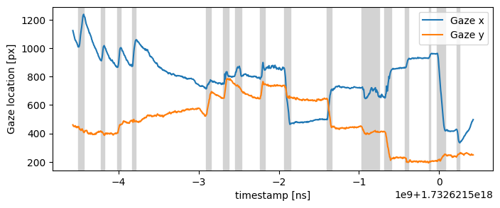
An example plot of cropped data#
Below we show how to easily plot the gaze and saccade data we cropped just now. Since PyNeon data are stored in pandas.DataFrame, you can use any plotting library that supports pandas.DataFrame as input. Here we use matplotlib to plot the gaze x, y coordinates and the saccade durations.
[13]:
import matplotlib.pyplot as plt

plt.figure(figsize=(8, 3))

# Plot the gaze data
(gaze_l,) = plt.plot(gaze_crop["gaze x [px]"], label="Gaze x")
(gaze_r,) = plt.plot(gaze_crop["gaze y [px]"], label="Gaze y")

# Visualize the saccades
for sac_start, sac_end in zip(saccades_crop.start_ts, saccades_crop.end_ts):
    sac = plt.axvspan(sac_start, sac_end, color="lightgray", label="Saccades")

plt.xlabel("Timestamp [ns]")
plt.ylabel("Gaze location [px]")
plt.legend(handles=[gaze_l, gaze_r, sac])
plt.show()
Visualizing gaze heatmap#
Finally, we will show how to plot a heatmap of the gaze/fixation data. Since it requires gaze, fixation, and video data, the input it takes is an instance of Recording that contains all necessary data. The method plot_heatmap(), by default, plots a gaze heatmap with fixations overlaid as circles.
[14]:
fig, ax = rec.plot_distribution()
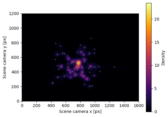
We can see a clear centre-bias, as participants tend to look more centrally relative to head position.