Reading Pupil Cloud-Format Recordings#
In this tutorial, we demonstrate how to load a Neon recording downloaded from Pupil Cloud and explore the data structure.
Downloading Sample Data#
We provide sample recordings in two formats:
Cloud format: Preprocessed data downloaded from Pupil Cloud with the “Timeseries Data + Scene Video” option
Native format: Raw data from the Neon companion device, also available via Pupil Cloud’s “Native Recording Data” option
This tutorial focuses on the cloud format. The API for accessing data is nearly identical across both formats.
Sample datasets can be conveniently downloaded using the get_sample_data() function, which returns a pathlib.Path object pointing to the downloaded and unzipped directory. PyNeon accepts both Path and string objects but internally uses Path for consistency.
[1]:
from pyneon import Dataset, Recording, get_sample_data

# Download sample data (if not existing) and return the path
sample_dir = get_sample_data("simple")
native_dir = sample_dir / "Native Recording Data"
cloud_dir = sample_dir / "Timeseries Data + Scene Video"
print(cloud_dir)
C:\Users\qian.chu\Documents\GitHub\PyNeon\data\simple\Timeseries Data + Scene Video
A dataset in cloud format has the following directory structure:
[2]:
from seedir import seedir

seedir(cloud_dir)
Timeseries Data + Scene Video/
├─enrichment_info.txt
├─sections.csv
├─simple1-56fcec49/
│ ├─3d_eye_states.csv
│ ├─blinks.csv
│ ├─events.csv
│ ├─fc7f4f44_0.0-8.235.mp4
│ ├─fixations.csv
│ ├─gaze.csv
│ ├─imu.csv
│ ├─info.json
│ ├─labels.csv
│ ├─saccades.csv
│ ├─scene_camera.json
│ ├─template.csv
│ └─world_timestamps.csv
└─simple2-6ca28606/
  ├─3d_eye_states.csv
  ├─7131b39b_0.0-6.654.mp4
  ├─blinks.csv
  ├─events.csv
  ├─fixations.csv
  ├─gaze.csv
  ├─gaze_data.csv
  ├─imu.csv
  ├─info.json
  ├─labels.csv
  ├─saccades.csv
  ├─scene_camera.json
  ├─template.csv
  ├─test.ipynb
  └─world_timestamps.csv
PyNeon provides a Dataset class to represent a collection of recordings. A dataset can contain one or more recordings. Here, we instantiate a Dataset by providing the path to the cloud format data directory.
[3]:
dataset = Dataset(cloud_dir)
print(dataset)
Dataset | 2 recordings
Dataset provides index-based access to its recordings through the recordings attribute, which contains a list of Recording instances. Individual recordings can be accessed by index:
[4]:
rec = dataset[0]  # Internally accesses the recordings attribute
print(type(rec))
print(rec.recording_dir)
print(rec)
<class 'pyneon.recording.Recording'>
C:\Users\qian.chu\Documents\GitHub\PyNeon\data\simple\Timeseries Data + Scene Video\simple1-56fcec49

Data format: cloud (version: 2.5)
Recording ID: 56fcec49-d660-4d67-b5ed-ba8a083a448a
Wearer ID: 028e4c69-f333-4751-af8c-84a09af079f5
Wearer name: Pilot
Recording start time: 2025-12-18 17:13:49.460000
Recording duration: 8235000000 ns (8.235 s)
Alternatively, you can directly load a single Recording by specifying the recording’s folder path:
[5]:
recording_dir = cloud_dir / "simple2-6ca28606"
rec = Recording(recording_dir)
print(type(rec))
print(rec.recording_dir)
print(rec)
<class 'pyneon.recording.Recording'>
C:\Users\qian.chu\Documents\GitHub\PyNeon\data\simple\Timeseries Data + Scene Video\simple2-6ca28606

Data format: cloud (version: 2.5)
Recording ID: 6ca28606-966d-486e-afe4-f4a424492d8c
Wearer ID: 028e4c69-f333-4751-af8c-84a09af079f5
Wearer name: Pilot
Recording start time: 2025-12-18 17:15:47.736000
Recording duration: 6654000000 ns (6.654 s)
Recording Metadata and Data Access#
You can quickly obtain an overview of a Recording by printing the instance. This displays basic metadata (recording ID, wearer ID, recording start time, and duration) and the paths to available data files. Note that at this point, data files are located but not yet loaded into memory.
[6]:
print(rec)
Data format: cloud (version: 2.5)
Recording ID: 6ca28606-966d-486e-afe4-f4a424492d8c
Wearer ID: 028e4c69-f333-4751-af8c-84a09af079f5
Wearer name: Pilot
Recording start time: 2025-12-18 17:15:47.736000
Recording duration: 6654000000 ns (6.654 s)
As shown in the output above, this recording contains all available data modalities. This tutorial focuses on non-video data; refer to the video processing tutorial for scene video analysis.
Individual data streams can be accessed as properties of the Recording instance. For example, recording.gaze retrieves gaze data and loads it into memory. If required files are missing, PyNeon raises a FileNotFoundError (and may warn about missing expected files).
[7]:
# Gaze and fixation data are available
gaze = rec.gaze
print(gaze)

saccades = rec.saccades
print(saccades)


scene_video = rec.scene_video
print(scene_video)
Stream type: gaze
Number of samples: 663
First timestamp: 1766074550059895270
Last timestamp: 1766074553373010270
Uniformly sampled: False
Duration: 3.31 seconds
Effective sampling frequency: 199.81 Hz
Nominal sampling frequency: 200 Hz
Columns: ['gaze x [px]', 'gaze y [px]', 'worn', 'fixation id', 'blink id', 'azimuth [deg]', 'elevation [deg]']

Events type: saccades
Number of samples: 8
Columns: ['start timestamp [ns]', 'end timestamp [ns]', 'duration [ms]', 'amplitude [px]', 'amplitude [deg]', 'mean velocity [px/s]', 'peak velocity [px/s]']

Video name: 7131b39b_0.0-6.654.mp4
Video height: 1200 px
Video width: 1600 px
Number of frames: 173
First timestamp: 1766074547736000000
Last timestamp: 1766074554369311111
Duration: 6.63 seconds
Effective FPS: 26.00
PyNeon reads tabular CSV files into specialized classes that inherit from two base classes: Stream and Events. All of these classes contain a data attribute that holds the tabular data as a pandas.DataFrame (reference).
Streamcontains continuous or semi-continuous data streams, including:Gaze (
Recording.gaze, fromgaze.csv)IMU (
Recording.imu, fromimu.csv)Eye states (
Recording.eye_states, from3d_eye_states.csv)Any other data stream that is indexed by timestamps in the same Unix nanosecond format
Eventscontains sparse event data (avoiding confusion with data fromevents.csv), including:Fixations (
Recording.fixations, fromfixations.csv)Saccades (
Recording.saccades, fromsaccades.csv)Blinks (
Recording.blinks, fromblinks.csv)Events (better thought of as messages/triggers,
Recording.events, fromevents.csv)Any other event data that is tabular and indexed by timestamps in the same Unix nanosecond format
Data Access as Pandas DataFrames#
The core of BaseTabular is the data attribute - a pandas.DataFrame that provides a standard Python data structure for tabular data manipulation. For example, you can view the first 5 rows using data.head() and inspect column data types with data.dtypes.
While you can reassign data to a separate variable, note that specialized processing methods operate at the class level and not on standalone DataFrames.
[8]:
print(gaze.data.head())
print(gaze.data.dtypes)
                     gaze x [px]  gaze y [px]  worn  fixation id  blink id  \
timestamp [ns]
1766074550059895270      777.823      645.708     1         <NA>      <NA>
1766074550064895270      778.840      650.667     1         <NA>      <NA>
1766074550069895270      789.575      644.583     1         <NA>      <NA>
1766074550075020270      790.720      643.566     1         <NA>      <NA>
1766074550080020270      788.473      642.554     1         <NA>      <NA>

                     azimuth [deg]  elevation [deg]
timestamp [ns]
1766074550059895270      -1.246504        -2.128223
1766074550064895270      -1.181023        -2.448048
1766074550069895270      -0.488220        -2.055796
1766074550075020270      -0.414293        -1.990205
1766074550080020270      -0.559308        -1.924897
gaze x [px]        float64
gaze y [px]        float64
worn                  Int8
fixation id          Int32
blink id             Int32
azimuth [deg]      float64
elevation [deg]    float64
dtype: object
[9]:
print(saccades.data.head())
print(saccades.data.dtypes)
            start timestamp [ns]   end timestamp [ns]  duration [ms]  \
saccade id
1            1766074550185020270  1766074550200020270             15
2            1766074550500394270  1766074550530409270             30
3            1766074550790643270  1766074550855643270             65
4            1766074551261017270  1766074551316141270             55
5            1766074551431266270  1766074551461266270             30

            amplitude [px]  amplitude [deg]  mean velocity [px/s]  \
saccade id
1                32.038345         2.058745           2169.577393
2                46.000240         2.955818           1558.823608
3               229.634521        14.681583           3085.043457
4               116.869461         7.418345           2315.360352
5                42.120010         2.639519           1429.373535

            peak velocity [px/s]
saccade id
1                    3185.151367
2                    1951.831299
3                    5698.534668
4                    3995.312500
5                    1764.324219
start timestamp [ns]      int64
end timestamp [ns]        int64
duration [ms]             Int64
amplitude [px]          float64
amplitude [deg]         float64
mean velocity [px/s]    float64
peak velocity [px/s]    float64
dtype: object
PyNeon performs the following preprocessing when reading CSV files:
Removes redundant
section idandrecording idcolumns present in the raw filesSets the
timestamp [ns](orstart timestamp [ns]for event files) column as the DataFrame indexAutomatically infers and assigns appropriate data types to columns—for example,
Int64for timestamps,Int32for event IDs, andfloat64for numerical measurements like gaze location and pupil size
Like any pandas.DataFrame, you can access individual rows, columns, or subsets using standard indexing and slicing methods. For example, data.iloc[0] returns the first row, and gaze['gaze x [px]'] (or equivalently gaze.data['gaze x [px]']) returns the gaze x-coordinate column.
[10]:
print(f"First row of gaze data:\n{gaze.data.iloc[0]}\n")
print(f"All gaze x values:\n{gaze['gaze x [px]']}")
First row of gaze data:
gaze x [px]         777.823
gaze y [px]         645.708
worn                    1.0
fixation id            <NA>
blink id               <NA>
azimuth [deg]     -1.246504
elevation [deg]   -2.128223
Name: 1766074550059895270, dtype: Float64

All gaze x values:
timestamp [ns]
1766074550059895270    777.823
1766074550064895270    778.840
1766074550069895270    789.575
1766074550075020270    790.720
1766074550080020270    788.473
                        ...
1766074553353010270    719.002
1766074553358010270    721.969
1766074553363010270    725.065
1766074553368010270    731.852
1766074553373010270    745.475
Name: gaze x [px], Length: 663, dtype: float64
Useful Properties and Methods for Streams and Events#
Beyond analyzing the data DataFrame directly, Stream and Events instances provide several convenience properties and methods for Neon-specific analysis. For instance, the ts property provides quick access to all timestamps as a numpy.ndarray (reference).
Unix timestamps in nanoseconds are typically inconvenient for human interpretation. PyNeon provides the times property, which represents relative time (in seconds) from the stream start—different from the recording start. Access this as a numpy.ndarray via the times property.
[11]:
print(f"First five timestamps:\n{gaze.ts[:5]}")
print(f"First five times:\n{gaze.times[:5]}")
First five timestamps:
[1766074550059895270 1766074550064895270 1766074550069895270
 1766074550075020270 1766074550080020270]
First five times:
[0.       0.005    0.01     0.015125 0.020125]
For a comprehensive list of available properties and methods, refer to the API reference documentation. Subsequent tutorials (for example, interpolation and concatenation of streams) demonstrate additional functionality.
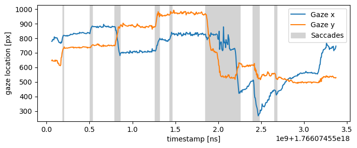
Example: Plotting Gaze and Saccade Data#
Below we demonstrate how to plot gaze and saccade data. Since PyNeon stores data in pandas.DataFrame format, you can use any plotting library that supports this structure. In this example, we use matplotlib to plot gaze coordinates and highlight saccade intervals.
[12]:
import matplotlib.pyplot as plt

plt.figure(figsize=(8, 3))

# Plot the gaze data
(gaze_l,) = plt.plot(gaze["gaze x [px]"], label="Gaze x")
(gaze_r,) = plt.plot(gaze["gaze y [px]"], label="Gaze y")

# Visualize the saccades
for sac_start, sac_end in zip(saccades.start_ts, saccades.end_ts):
    sac = plt.axvspan(sac_start, sac_end, color="lightgray", label="Saccades")

plt.xlabel("timestamp [ns]")
plt.ylabel("gaze location [px]")
plt.legend(handles=[gaze_l, gaze_r, sac])
plt.show()
Visualizing Gaze Distribution#
To visualize the spatial distribution of gaze data, we can create a heatmap with fixation locations overlaid. The plot_distribution() method generates this visualization by combining gaze density with fixation markers.
[13]:
fig, ax = rec.plot_distribution()
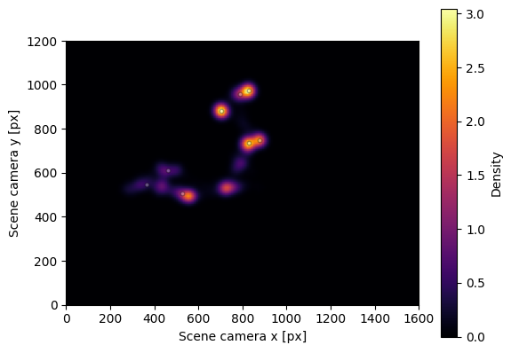
The plot appears relatively sparse due to the short duration of this sample recording. For longer recordings with more gaze samples, plot_distribution() provides a valuable tool for visualizing gaze and fixation patterns across the scene.