Surface Mapping Using Fiducial Markers and Screen Corners#
What are Fiducial Markers?#
Fiducial markers (for a review see 1) are specially designed visual patterns that serve as reference points for establishing coordinate correspondence. They are reliably detected in images, enabling transformation between image/video coordinates and real-world coordinates. In eye-tracking, they allow us to transform gaze from the camera’s perspective to the observed surface (for example, a computer screen).
PyNeon supports two widely-adopted marker systems:
AprilTag (references2,3): Also used by Pupil Labs Neon Player and Pupil Cloud.
ArUco (reference4): Integrated into OpenCV, enabling marker detection via cv2.aruco.

Sample Dataset#
We use a sample dataset called “markers” containing two recordings: one with AprilTag markers and one with ArUco markers. In both, a participant viewed artworks on a computer screen. Specifically, the participant moved their head often to test robustness under larger head motion. We will map gaze and fixation data onto the screen using markers visible in the scene video. The sample data is fetched via get_sample_data(...) and stored locally after download.
[1]:
from pyneon import Dataset, get_sample_data
import matplotlib.pyplot as plt

# Load a sample recording
dataset_dir = get_sample_data("markers", format="cloud")
dataset = Dataset(dataset_dir)
Let’s start with the AprilTag recording (recording index 0).
[2]:
rec = dataset.recordings[0]
print(rec)
Data format: cloud (version: 2.5)
Recording ID: 16841adb-da58-4c42-be02-f052c3c43db3
Wearer ID: 028e4c69-f333-4751-af8c-84a09af079f5
Wearer name: Pilot
Recording start time: 2025-09-22 00:25:14.096000
Recording duration: 244820000000 ns (244.82 s)
AprilTag Example#
Visualizing Markers in Video#
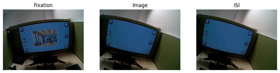
First, inspect a few frames to confirm the markers are clearly visible and well lit. Below are three example frames: fixation cross, artwork presentation, and inter-trial interval.
[3]:
video = rec.scene_video

fig, axs = plt.subplots(1, 3, figsize=(12, 3))
video.plot_frame(380, ax=axs[0], show=False)
video.plot_frame(500, ax=axs[1], show=False)
video.plot_frame(520, ax=axs[2], show=False)
axs[0].set_title("Fixation")
axs[1].set_title("Image")
axs[2].set_title("ISI")
plt.show()
Step 1: Detect Markers#
The detect_markers() method automatically detects AprilTag or ArUco markers. The only required argument is marker_family (for example, '36h11' for AprilTag tag36h11, omitting “tag”).
Optional parameters allow customization:
processing_window: restrict detection to a specific time rangeprocessing_window_unit: interpret the window as frames, seconds, or timestampsstep: process every Nth frame to speed up detectiondetector_parameters: pass customcv2.aruco.DetectorParametersfor fine-tuningundistort: optionally undistort frames before detection
Here we use default settings, processing all frames:
[4]:
from pathlib import Path
from pyneon import Stream
import os

detection_path = Path("export") / "detected_markers.csv"
if detection_path.exists():
    detected_markers = Stream(detection_path)
else:
    os.makedirs(detection_path.parent, exist_ok=True)
    detected_markers = video.detect_markers("36h11", step=5)
    detected_markers.save(detection_path)
Verifying Detection#
Detected markers are stored in a PyNeon Stream with timestamps from the video frames. Each row corresponds to a detection and includes the marker id and corner coordinates in the video frame.
[5]:
print(detected_markers.data.head(20))
                     frame index marker family marker id marker name  \
timestamp [ns]
1758493517123422222           65         36h11         0     36h11_0
1758493517123422222           65         36h11         5     36h11_5
1758493517123422222           65         36h11         4     36h11_4
1758493517623233333           80         36h11         0     36h11_0
1758493517623233333           80         36h11         1     36h11_1
1758493517623233333           80         36h11         2     36h11_2
1758493517623233333           80         36h11         5     36h11_5
1758493517623233333           80         36h11         4     36h11_4
1758493517623233333           80         36h11         3     36h11_3
1758493517789844444           85         36h11         0     36h11_0
1758493517789844444           85         36h11         1     36h11_1
1758493517789844444           85         36h11         5     36h11_5
1758493517789844444           85         36h11         2     36h11_2
1758493517789844444           85         36h11         4     36h11_4
1758493517789844444           85         36h11         3     36h11_3
1758493517956444444           90         36h11         0     36h11_0
1758493517956444444           90         36h11         1     36h11_1
1758493517956444444           90         36h11         2     36h11_2
1758493517956444444           90         36h11         5     36h11_5
1758493517956444444           90         36h11         4     36h11_4

                     top left x [px]  top left y [px]  top right x [px]  \
timestamp [ns]
1758493517123422222            969.0            200.0            1031.0
1758493517123422222            991.0            380.0            1050.0
1758493517123422222           1008.0            546.0            1063.0
1758493517623233333            443.0            539.0             502.0
1758493517623233333           1201.0            482.0            1259.0
1758493517623233333           1204.0            672.0            1261.0
1758493517623233333            467.0            722.0             525.0
1758493517623233333            497.0            888.0             552.0
1758493517623233333           1198.0            846.0            1252.0
1758493517789844444            403.0            535.0             465.0
1758493517789844444           1182.0            458.0            1242.0
1758493517789844444            433.0            723.0             493.0
1758493517789844444           1188.0            653.0            1247.0
1758493517789844444            470.0            893.0             527.0
1758493517789844444           1185.0            830.0            1241.0
1758493517956444444            358.0            531.0             420.0
1758493517956444444           1152.0            448.0            1213.0
1758493517956444444           1159.0            645.0            1219.0
1758493517956444444            392.0            722.0             451.0
1758493517956444444            431.0            895.0             489.0

                     top right y [px]  bottom right x [px]  \
timestamp [ns]
1758493517123422222             192.0               1037.0
1758493517123422222             377.0               1055.0
1758493517123422222             547.0               1067.0
1758493517623233333             533.0                509.0
1758493517623233333             480.0               1260.0
1758493517623233333             666.0               1259.0
1758493517623233333             720.0                534.0
1758493517623233333             888.0                563.0
1758493517623233333             837.0               1247.0
1758493517789844444             526.0                473.0
1758493517789844444             455.0               1245.0
1758493517789844444             719.0                504.0
1758493517789844444             646.0               1246.0
1758493517789844444             892.0                539.0
1758493517789844444             820.0               1237.0
1758493517956444444             522.0                431.0
1758493517956444444             445.0               1216.0
1758493517956444444             638.0               1218.0
1758493517956444444             718.0                463.0
1758493517956444444             894.0                503.0

                     bottom right y [px]  bottom left x [px]  \
timestamp [ns]
1758493517123422222                257.0               976.0
1758493517123422222                438.0               997.0
1758493517123422222                600.0              1010.0
1758493517623233333                599.0               450.0
1758493517623233333                546.0              1203.0
1758493517623233333                727.0              1202.0
1758493517623233333                780.0               477.0
1758493517623233333                942.0               508.0
1758493517623233333                890.0              1192.0
1758493517789844444                593.0               412.0
1758493517789844444                521.0              1186.0
1758493517789844444                780.0               444.0
1758493517789844444                708.0              1189.0
1758493517789844444                944.0               483.0
1758493517789844444                873.0              1183.0
1758493517956444444                592.0               370.0
1758493517956444444                513.0              1155.0
1758493517956444444                701.0              1160.0
1758493517956444444                781.0               403.0
1758493517956444444                948.0               445.0

                     bottom left y [px]  center x [px]  center y [px]
timestamp [ns]
1758493517123422222               262.0        1003.25         227.75
1758493517123422222               438.0        1023.25         408.25
1758493517123422222               598.0        1037.00         572.75
1758493517623233333               604.0         476.00         568.75
1758493517623233333               550.0        1230.75         514.50
1758493517623233333               734.0        1231.50         699.75
1758493517623233333               783.0         500.75         751.25
1758493517623233333               941.0         530.00         914.75
1758493517623233333               898.0        1222.25         867.75
1758493517789844444               600.0         438.25         563.50
1758493517789844444               526.0        1213.75         490.00
1758493517789844444               784.0         468.50         751.50
1758493517789844444               716.0        1217.50         680.75
1758493517789844444               947.0         504.75         919.00
1758493517789844444               884.0        1211.50         851.75
1758493517956444444               597.0         394.75         560.50
1758493517956444444               517.0        1184.00         480.75
1758493517956444444               709.0        1189.00         673.25
1758493517956444444               783.0         427.25         751.00
1758493517956444444               947.0         467.00         921.00
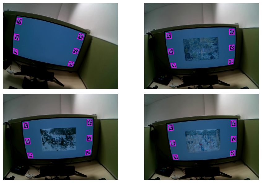
Spot-check detections by plotting markers on selected frames. This makes it easy to confirm that ids are correct and corners line up with the visual markers:
[6]:
# Plot a few frames with detected markers
fig, axs = plt.subplots(2, 2, figsize=(10, 6), tight_layout=True)
axs = axs.flatten()
video.plot_detections(detected_markers, frame_index=500, ax=axs[0], show=False)
video.plot_detections(detected_markers, frame_index=1000, ax=axs[1], show=False)
video.plot_detections(detected_markers, frame_index=1500, ax=axs[2], show=False)
video.plot_detections(detected_markers, frame_index=2000, ax=axs[3], show=False)
plt.show()
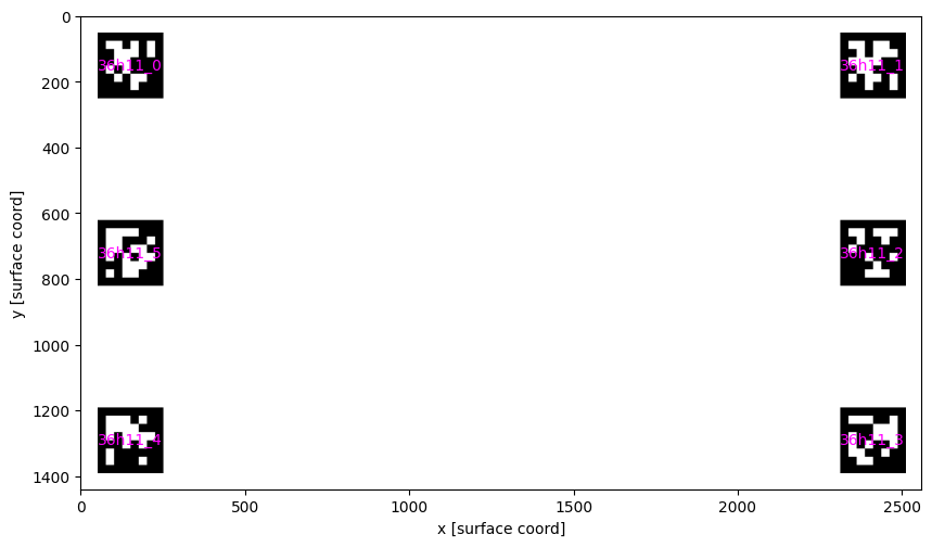
Step 2: Define Real-World Marker Coordinates#
To establish the mapping, provide a dataframe with real-world coordinates for each marker. This requires:
Marker name: must match the ids reported by
detect_markers()Center coordinates: where the marker is located in the target surface coordinate system (here, screen pixels)
Size: physical marker size in the same units as the target surface
In this experiment (screen resolution 2560x1440), markers were placed near the screen corners with a 50 px margin and 200x200 px size. They are also placed in a clockwise order, starting from the top-left corner.
Once a marker_info dataframe is defined, we can preview it to make sure the coordinates look correct using the plot_marker_layout() function:
[7]:
from pyneon.vis import plot_marker_layout
import pandas as pd

width = 2560
height = 1440
marker_layout = pd.DataFrame(
    {
        "marker name": [f"36h11_{i}" for i in range(6)],
        "size": 200,
        "center x": [150, width - 150, width - 150, width - 150, 150, 150],
        "center y": [150, 150, height / 2, height - 150, height - 150, height / 2],
    }
)
print(marker_layout)

fig, ax = plt.subplots(figsize=(10, 6))
plot_marker_layout(marker_layout, ax=ax, show_marker_names=True, show=False)
ax.set_xlim(0, width)
ax.set_ylim(height, 0)
plt.show()
  marker name  size  center x  center y
0     36h11_0   200       150     150.0
1     36h11_1   200      2410     150.0
2     36h11_2   200      2410     720.0
3     36h11_3   200      2410    1290.0
4     36h11_4   200       150    1290.0
5     36h11_5   200       150     720.0
Step 3: Compute Homography Transformation#
The find_homographies() method computes a frame-by-frame 2D transformation (homography) between detected marker locations and their real-world coordinates. The result is a Stream of 3x3 homography matrices, one per frame where enough markers are available. These matrices enable mapping any point from camera coordinates to screen coordinates.
[8]:
from pyneon.video import find_homographies

homographies = find_homographies(
    detected_markers,
    layout=marker_layout,
)
print(homographies.data.head())
Computing surface-mapping homographies: 100%|██████████| 1408/1408 [00:02<00:00, 650.41it/s]
                     homography (0,0)  homography (0,1)  homography (0,2)  \
timestamp [ns]
1758493517123422222          5.314940         -0.583451      -4959.439257
1758493517623233333          2.598597         -0.442606       -850.410264
1758493517789844444          2.466307         -0.499194       -665.028851
1758493517956444444          2.398689         -0.518810       -521.535770
1758493518123044444          2.349698         -0.485569       -470.320079

                     homography (1,0)  homography (1,1)  homography (1,2)  \
timestamp [ns]
1758493517123422222          0.617168          4.761420      -1464.540605
1758493517623233333          0.186317          2.581638      -1427.930238
1758493517789844444          0.231569          2.461035      -1360.495722
1758493517956444444          0.241472          2.405991      -1316.174140
1758493518123044444          0.238705          2.379632      -1263.913540

                     homography (2,0)  homography (2,1)  homography (2,2)
timestamp [ns]
1758493517123422222          0.000712         -0.000454               1.0
1758493517623233333         -0.000007         -0.000212               1.0
1758493517789844444         -0.000023         -0.000216               1.0
1758493517956444444         -0.000029         -0.000218               1.0
1758493518123044444         -0.000047         -0.000200               1.0
Step 4: Apply Transformation to Gaze Data#
Now apply the homography transformation to project gaze and fixations onto screen coordinates. This is done using the apply_homographies() method of gaze and fixation objects. Internally, PyNeon interpolates the homographies to the timestamps of the gaze and fixation samples and applies the closest valid transform.
You might notice warning messages. They are expected when homographies are missing for some frames (for example, markers were not visible or were blurred). If the nearest homography is too far from a sample time (default 500 ms), the sample is dropped. You can change this behavior with the max_gap_ms argument.
[9]:
gaze_on_surface = rec.gaze.apply_homographies(homographies)
fixations_on_surface = rec.fixations.apply_homographies(homographies)
C:\Users\qian.chu\Documents\GitHub\PyNeon\pyneon\preprocess\preprocess.py:67: UserWarning: 134 out of 48219 requested timestamps are outside the data time range and will have empty data.
  warn(
C:\Users\qian.chu\Documents\GitHub\PyNeon\pyneon\preprocess\preprocess.py:110: UserWarning: 601 out of 48219 requested timestamps exceed max_gap_ms=500 relative to neighboring samples and will have empty data.
  warn(
Applying homographies to gaze points: 100%|██████████| 47484/47484 [00:27<00:00, 1695.94it/s]
C:\Users\qian.chu\Documents\GitHub\PyNeon\pyneon\preprocess\preprocess.py:67: UserWarning: 1 out of 476 requested timestamps are outside the data time range and will have empty data.
  warn(
C:\Users\qian.chu\Documents\GitHub\PyNeon\pyneon\preprocess\preprocess.py:110: UserWarning: 9 out of 476 requested timestamps exceed max_gap_ms=500 relative to neighboring samples and will have empty data.
  warn(
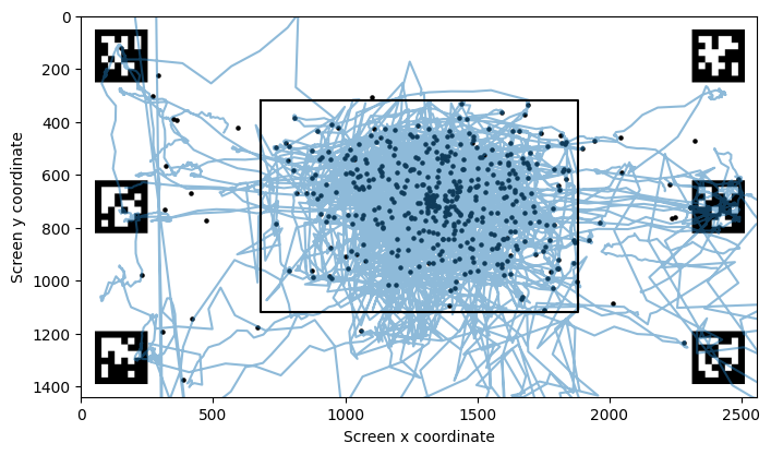
Now let’s plot all the mapped gaze and fixation data in the screen’s reference frame (origin at top-left, y increases downward):
[10]:
fig, ax = plt.subplots(figsize=(8, 6))
plot_marker_layout(marker_layout, ax=ax, show_marker_names=False, show=False)
ax.plot(
    gaze_on_surface.data["gaze x [surface coord]"],
    gaze_on_surface.data["gaze y [surface coord]"],
    alpha=0.5,
)

ax.scatter(
    fixations_on_surface.data["fixation x [surface coord]"],
    fixations_on_surface.data["fixation y [surface coord]"],
    s=5,
    c="black",
)

# Plot where the artworks were
# There were 1200 x 800 pixels in size, centered on the screen (2560 x 1440)
ax.plot(
    [680, 1880, 1880, 680, 680],
    [320, 320, 1120, 1120, 320],
    color="black",
    label="Image outline",
)

ax.set_xlabel("Screen x coordinate")
ax.set_ylabel("Screen y coordinate")

ax.set_xlim(0, 2560)
ax.set_ylim(0, 1440)
ax.invert_yaxis()
plt.show()
Example 2: ArUco Markers#
The same workflow applies to ArUco markers. Instead of a family name, ArUco dictionaries are specified by their pattern (for example, '5x5_50'). The same four steps (detect, define coordinates, compute homography, transform) apply; only the marker family changes.
[11]:
rec = dataset.recordings[1]
video = rec.scene_video
detected_markers = video.detect_markers("5x5_50")
Detecting markers:   0%|          | 0/1044 [00:00<?, ?it/s]C:\Users\qian.chu\Documents\GitHub\PyNeon\pyneon\video\video.py:409: UserWarning: Failed to retrieve frame at index 0. Returning None.
  warn(f"Failed to retrieve frame at index {frame_index}. Returning None.")
Detecting markers: 100%|██████████| 1044/1044 [00:08<00:00, 120.82it/s]
Using the shorter ArUco video, we will visualize detections across the full recording. Set show_video=False to avoid the interactive preview window and instead save the overlay to output_path.
[12]:
video.overlay_detections(
    detected_markers, show_video=False, output_path="export/marker_detections.mp4"
)
Overlaying detections on video:   0%|          | 0/1044 [00:00<?, ?it/s]C:\Users\qian.chu\Documents\GitHub\PyNeon\pyneon\video\video.py:409: UserWarning: Failed to retrieve frame at index 0. Returning None.
  warn(f"Failed to retrieve frame at index {frame_index}. Returning None.")
Overlaying detections on video: 100%|██████████| 1044/1044 [00:08<00:00, 126.95it/s]
Alternative: Contour-Based Screen-Corner Detection#
When fiducial markers are unavailable, estimate the homography from bright screen corners. The detect_contour() method looks for a bright rectangular contour per frame and returns its four corners. This works best when the screen is brighter than the background. You can tune brightness_threshold, adaptive, or morph_kernel, and use step or processing_window to speed up processing.
[13]:
import numpy as np
from pyneon.video import find_homographies

screen_detections = video.detect_contour()

contour_layout = np.array(
    [
        [0, 0],
        [width, 0],
        [width, height],
        [0, height],
    ],
    dtype=np.float32,
)

homographies_screen = find_homographies(
    screen_detections,
    layout=contour_layout,
)
Detecting contour corners:   0%|          | 0/1044 [00:00<?, ?it/s]C:\Users\qian.chu\Documents\GitHub\PyNeon\pyneon\video\video.py:409: UserWarning: Failed to retrieve frame at index 0. Returning None.
  warn(f"Failed to retrieve frame at index {frame_index}. Returning None.")
Detecting contour corners: 100%|██████████| 1044/1044 [00:07<00:00, 135.31it/s]
Computing surface-mapping homographies: 100%|██████████| 870/870 [00:00<00:00, 2685.67it/s]
[14]:
video.plot_detections(screen_detections, 500)
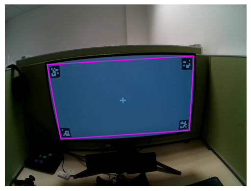
[14]:
(<Figure size 640x480 with 1 Axes>, <Axes: >)
[15]:
video.overlay_detections(
    screen_detections,
    show_video=False,
    show_ids=False,
    output_path="export/contour_detections.mp4",
)
Overlaying detections on video:   0%|          | 0/1044 [00:00<?, ?it/s]C:\Users\qian.chu\Documents\GitHub\PyNeon\pyneon\video\video.py:409: UserWarning: Failed to retrieve frame at index 0. Returning None.
  warn(f"Failed to retrieve frame at index {frame_index}. Returning None.")
Overlaying detections on video: 100%|██████████| 1044/1044 [00:08<00:00, 117.43it/s]